What kind of thing is MEGA?
To borrow from my first blog post: MEGA, at its core, is a Genetic Algorithm, yet it couldn’t be further from a Standard GA (SGA). So much so that I argue that it is in fact its own class of algorithm.
Below, I’m going to walk you through a high-level overview of how MEGA maintains the core functionality of an SGA while being categorically different from other Evolutionary Algorithms. This is not an in-depth technical walkthrough. It is intended to build intuition about how MEGA functions before taking a technical deep dive.
This document is quite necessarily long, 25 pages to be exact. I realize this might be a bit much for most people but to help make it a bit more manageable you can download a PDF version of the document
here >(What Kind of Thing is MEGA).
Why take this approach?
Because there are a lot of nuances that are easy to misunderstand without a conceptual intuition for what makes MEGA distinct. If you look at the components in isolation, they might appear to be standard features. It is only when you see how they interact—how one mechanism creates a problem that the next mechanism solves—that the system makes sense.
For this reason, this document is written as a constructive narrative. We will start with the basic mechanics and then introduce failure modes as they naturally arise. We will then introduce the specific MEGA mechanisms that exist solely to resolve those failures.
I recommend reading this in in full. The dynamics of the later sections rely entirely on the context established in the earlier sections. If you skip ahead or skim, you risk seeing the how without understanding the why, which misses the point entirely.
Even if your goal is technical depth, I recommend reading this first. MEGA’s internal dynamics are fairly complex, and the logic behind them is not always obvious until you see the problems they were designed to fix.
MEGA follows the typical SGA loop
Initialize Encoding and other parameters > Initial Population > Evaluate > Select Parents > Breed and Mutate Parents > Exit If: solution or generation count meets criteria > Else: Go to Evaluate.
The core of MEGA’s divergence from an SGA comes from its encoding conventions and mutation operators. These, in turn, require additional mechanisms to manage the complexity that emerges from evolving representations.
How the encodings work
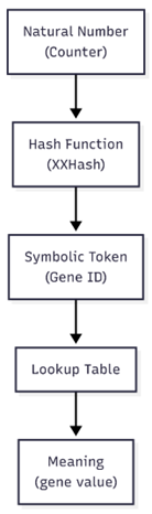
The mechanics here are straightforward, but the consequences are not. When a gene is added, a counter is incremented if we need a new encoding. The value of the counter is given to a 64-bit Hash function XXHash to generate its hash token. The hash function is noncryptographic and is used as a unique identifier to look up mappings. The hash can then be used as the identifier to “decode” the encoding back to its value. So, gene encodings are essentially hashes of natural numbers in ascending order. The hash is used purely as a unique identifier for efficient lookup; decoding is performed via an internal mapping, not by inverting the hash.
Although gene identifiers are generated from integers, they should be understood as discrete symbolic tokens rather than numeric values. No ordering, continuity, or metric structure is assumed or used. This may change in future versions of MEGA as it evolves over time but as of now, genes in MEGA are as described above. Gene identifiers can be thought of as Gene1, Gene2, Gene3, etc. Hashing is for the sake of efficiency in lookup, nothing more.
Note: Genes are treated as atomic symbols, not numbers. The number 7 is not ‘closer’ to the number 8 than it is to the number 100. This is for the sake of having a unique identifier for each gene, not counting or ordering.
Mutations
Ok so let’s move on to mutations, this is where the interesting bits happen (pun intended). When making a mutation pass, we check each index in an encoded solution and perform a mutation roll which is a random roll with an output value between 0 and 1. The mutation roll is a way of checking each gene in the solution and saying, ‘Do I mutate this gene or not?’ according to some parameter-defined probability. First, I will lay out the typical SGA mutations that MEGA uses and then I will introduce the new MEGA-specific mutations.
It should be noted that there are two different mutation rates that govern the frequency of the SGA mutations. When a gene index is selected for an SGA mutation the exact mutation applied is selected randomly from among the available options.
SGA Mutations that MEGA also uses:
- Swap: Swaps the gene being mutated with a neighbor randomly selected to the left or right. Allows for genes to migrate through the solution over time.
- Point: Replaces the Gene being mutated with a new gene from the gene pool selected at random. This allows for new information to enter the population.
- Insert: Inserts a gene randomly selected from the gene pool at a position randomly selected to the left or the right of the gene being mutated. This allows for new information to enter the population without overwriting.
- Delete: Deletes the gene being mutated. Allows for information to be removed from the population.
Note: All SGA mutations serve their typical function with the exception that they are also modified with MEGA-specific limitations that influence their behavior under certain circumstances which will all be addressed and explained as we go.
Ok, now let’s look at the MEGA-specific mutations and how they work. This isn’t going to be a pretty list with a one-sentence explanation because these mutations have rules and context that limit where they can be used under what circumstances. Before that though we need to explain two special genes that are part of every MEGA instance regardless of application. They are the Start and End delimiters. They can be thought of as ( and ), respectively. In fact, for the sake of simplicity, that is how they will be represented through this post.
Note: From here on out this is where things begin to diverge significantly from the SGA paradigm.
- Delimiters have no meaning in the context of evaluation of a solution; they only matter to mutation and crossover.
- Delimiters can be seen as atomic pairs. They are created in pairs, mutations respect their ordering, and crossover is forbidden from happening within them.
- Over time, delimiters can come to encapsulate sections of the solution sequence. However, each ( must be properly closed by ) with no other delimiters inside.
- Delimiters modify the mutation rates when the mutation index crosses into their boundaries and allow for or exclude certain mutation types that can be applied to the content they encapsulate.
So how do delimiters come to exist within the population? This would be the first MEGA-specific mutation, insert delimiter pair, which has its own probability parameter. Like other mutations, it is applied probabilistically. Delimiters cannot be inserted between other delimiters as this would potentially disrupt their ordering.
Say we have sequence ABC(DEFG)HIJ. If we try to insert a delimiter pair inside of (DEFG) say, to delimit EF we end up with (D(EF)G). In mathematics, this makes sense: handle (EF) first before the outer brackets. However, in MEGA delimiters are expected to not have nesting, at least not in this form. MEGA does support hierarchy, but not through arbitrary nesting of delimiters. That distinction becomes important once Capture is introduced. Before we get into that though we need to go back to the swap mutation to explain its rule regarding acting on delimiters.
The swap mutation, as noted above, is applied to a gene at a certain index it randomly chooses swap left or right then swaps the gene being mutated with the adjacent gene in the chosen direction. Take sequence ABC if B has a swap mutation applied to the left, then the resulting sequence will be BAC.
So how does this apply to delimiters?
Example:
Say we have sequence AB(CDE)(FG)HIJ and a swap mutation is triggered on the first (between B and C, it’s a swap to the left again. The resulting sequence would be A(BCDE)(FG)HIJ this is a valid swap mutation. Now let’s say another swap mutation occurs on the delimiter after E and it’s to the right the resulting solution would be A(BCDE()FG)HIJ this results in an invalid ordering of delimiters because we have (content(), which is a violation of delimiter ordering, which is why the swap rules forbid swapping two delimiters; to preserve ordering.
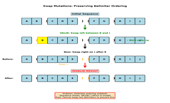
In summary
Insert delimiter pair is a probabilistic mutation that introduces new, ordered structure into solutions. Delimiters are strictly ordered as (content) and cannot be nested. This ordering constraint forbids delimiter–delimiter swaps while still allowing delimiters to move relative to non-delimiter genes. The result is structure that can form and migrate (through swap mutations) but not collapse into ambiguity.
The next MEGA-specific mutation we will introduce is the Capture mutation. You might have noticed, when explaining encodings, that it is implied that new genes can come to exist over the run. This is accomplished through the capture mutation which is fairly straightforward. Let’s suppose that we are mutating sequence ABC(DEFG)HIJ. As the index of the gene being checked for mutation passes the ( gene, the capture mutation becomes an option and is subject to its own independent probability of occurring until the mutation index leaves the ) delimiter. If a capture mutation occurs anywhere on or within the delimiter pair (DEFG) the delimiters and their content are removed, and metagene is created which contains the content of those delimiters.
Example:
Let’s consider AB(CDE)(FG)HIJ again. If there is a capture mutation anywhere in the (CDE) sequence a new metagene M1 is created, and the new sequence would become AB M1 (FG)HIJ, which at evaluation would decode to ABCDE(FG)HIJ. Notice the ( ) that encapsulated CDE are not present, yet the gene sequence ABCDEFGHIJ remains intact. It’s also worth noting that decoding sequences in MEGA can optionally be set to return delimiters that haven’t been captured yet in the decoded solution. So, the decoded solution could also be ABCDE(FG)HIJ.
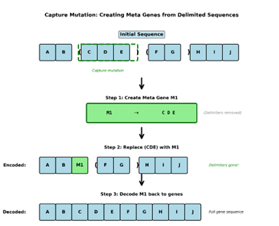
Up until now genes have been referred to as just genes and delimiters but we can now make a distinction between types of genes. Delimiters are technically genes, but they don’t matter to fitness evaluation, so they are essentially invisible to anything but mutation and crossover. They serve as structural markers that create boundaries that modify the mutation behavior of the system. The real distinction comes between Base genes and metagenes. Base genes are the basic set of genes that exist after initialization. The Encodings cover the two Delimiters and the set of base genes. In the case of our example ( => gene 1, )=> gene2, A=> gene3, …, J=> gene12. That is our set of base genes. Now we just triggered the creation of a new Metagene which consists of the content CDE: gene13 if we’re counting, but for simplicity let’s refer to it as M1.
Let’s return to delimiter nesting for a moment now that we have a firm concept of how the capture mutation behaves. Nested delimiters are excluded not as a stylistic constraint, but because metagenes are destructive abstractions that replace their contents. Allowing nested delimiters would introduce ambiguity in capture order: inner regions would need to be captured before outer regions, requiring additional mutation regimes, ordering rules, and representational bookkeeping. This would collapse the clean separation between structural stabilization and representational compression that MEGA relies on. By forbidding nesting, capture remains order-independent and well-defined.
Note: The area within delimiters is referred to as a delimited region and the area outside of delimiters is referred to as an undelimited region.
Now that we have properly defined delimiters Base genes and metagenes, we can begin to see a glimpse of the dynamics that are being allowed to emerge. Before we go further, I think it is necessary to briefly explain the intuition and necessity behind delimiters and their rules.
The first important thing to keep in mind is that delimited regions are subject to a different mutation rate and set of mutations than undelimited regions.
Next crossover is forbidden from occurring where the cut points are within delimiters. This means that crossover is constrained to only happen within undelimited regions.
These two constraints work together to address a known and well documented limitation of SGA. You can read about it in the paper, ”The Royal Road for Genetic Algorithms: Fitness Landscapes and GA Performance,” where researchers directly test the assertions of Schema theory and the Building Blocks hypothesis.
Delimiters and the constraints they impose work to address the issue of disrupting intermediate schema through a process that is almost more physical-like than informational. Physical in the dynamical sense: persistence emerges from asymmetric transformation rates across a boundary, not from symbolic interpretation. The lower differential mutation rate within delimited regions creates a region of stability within solutions. Through swap mutations, these regions are malleable; able to be expanded, contracted, and shifted within solutions. This mobile island of stability will come to encapsulate important information due to the simple fact that solutions that don’t protect important information will lose it due to the disruption of mutation, leading to them not surviving. This is further reinforced by the disruptive effects of crossover; whereas a sequence increases in length it becomes increasingly likely that it will be broken or disrupted through crossover. Delimiters address this through explicitly forbidding crossover cut points from happening within them.
All of that comes together to show and explain how delimiters come to encapsulate information that is important to the survival of solutions within the population. As delimited regions reproduce within the population the information they contain comes to have an increased probability of having a capture mutation happen within them leading to their information being used in the creation of new metagenes.
The capture mutation has two rules:
- Exact duplicates of metagene content are not allowed. So once a sequence is captured no other metagenes will be created that contain an identical sequence of encodings as the original.
Note: This is not the same as decoding to an identical base gene sequence. The disallowing of duplicates is primarily about structure not outcome. This will be important once nesting is explained.
- Capture is restricted from capturing delimited regions that are less than two genes long as this would be redundant and counterproductive.
This is the first point at which MEGAs representational hierarchy begins to form. We can now address the MEGA-specific rules regarding point and insert mutations and how they enable the creation of an evolved hierarchical representation.
Once metagenes exist within the population, they become available for use anywhere via point and insert mutations.
Let’s assume, for a moment, that point and insert mutations behave in MEGA exactly as they do in a standard GA. As metagenes are added to the gene pool, the probability that a randomly selected gene will be a metagene increases.
This creates a runaway effect. As metagene usage increases, the system rapidly loses its ability to make small, local changes through Base genes. Variation becomes coarse-grained, dominated by large representational substitutions. The result is uncontrolled representational bloat, loss of fine-grained adaptation, and eventual population collapse.
This failure mode is not incidental; it is structurally guaranteed if metagenes are treated blindly the same as Base genes.
Preventing this collapse requires additional rules governing how point and insert mutations may introduce metagenes. These rules are not arbitrary constraints, but necessary conditions for maintaining a balance between abstraction and variation. It is through these constraints that MEGA’s hierarchical representation remains both expressive and stable.
An example of this is: say we start out with a set of 3 Base genes. When a mutation randomly selects a base gene, each base gene has a 1 in 3 chance of being used. If we create a metagene and apply gene selection uniformly then each base gene now has a 1 in 4 chance. Add another 1 in 5, another, 1 in 6. As we go on, the probability of any single base gene being selected slowly vanishes giving way to the system favoring coarse-grained metagenes.
The solution to this is pretty straightforward. We introduce a new probability that dictates the choice between metagene and base gene. This gives us control over how aggressively we favor metagene reuse over base gene usage.
Another way of looking at this could be how recursive the system is. Since point and insert mutations are allowed within delimited regions, metagenes can themselves come to contain other metagenes. This is how the hierarchical representational data structure emerges. This is called the Metagenome. It can also be seen as a form of recursion.
Delimiters don’t nest as stated above. Metagenes however can. The hierarchy is in the captured tokens, not in the nesting parentheses. Just as a base gene being used within a metagene doesn’t remove it from being used as a unique unit. Metagenes can be used as units within delimiters and ultimately be captured. Creating the hierarchical nesting we leverage to enable the rest of MEGAS dynamics. The metagenome represents a decoding mapping from genotype to phenotype (how to go from encoded solution to the decoded solution). This data structure is what is commonly referred to as a Directed Acyclic Graph (DAG) in Graph Theory.
My aim here is to avoid formal mathematics in this write-up, but this is one place where a precise term is unavoidable. The metagenome is, formally speaking, a Directed Acyclic Graph (DAG).
The problem is that DAGs are usually introduced as static mathematical objects, and if a non-technical reader looks the term up (or follows the above link) they will almost certainly disappear down a rabbit hole that is not relevant to what is happening here. That is not what I mean by invoking the term.
What matters for intuition are a small number of structural properties: Metagenes can reference earlier genes, those dependencies always flow in one direction, and circular self-reference is impossible. These constraints are what make metagene nesting meaningful rather than flat. Without them, hierarchy collapses into a loose collection of macros with no real structure.
Some of the deeper mathematical consequences of DAGs may also apply to the metagenome, but I have not explored those implications fully yet. The purpose of introducing the term here is not to make a formal graph-theoretic claim, but to clearly establish the structural rules that are known to apply and that are essential for understanding how the metagenome functions and evolves inside MEGA.
So let’s get into how the evolution of the metagenome comes to construct a DAG-like structure without diving too deeply into the hard Graph Theory.
Example:
When the algorithm is first initialized, we have: (let’s use our base gene set from above ABCDEFGHIJ). Next our example captured a new metagene M1 which is composed of CDE and that is where we stopped. It was mentioned that metagenes can then be nested within other metagenes through usage, but we didn’t have a specific example. So, let’s say that a new delimited sequence forms, consisting of (AB M1 D) which is captured and creates a new metagene M2 composed of AB M1 D. Note: I’m using the real values of the genes and not their encodings for simplicity.
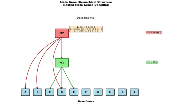
Now we need to decode this gene so first we look at the mapping of the M2 metagenes encoding to its content which gives us back AB M1 D. The first value is A, the second is B, then we hit the nested metagene M1. M1 then gets sent back to the decoder to look up its values which gives us back CDE. CDE is concatenated to the original AB to make ABCDE. Next, we look at the last gene, which is D. This is then concatenated to the ABCDE. Giving us ABCDED and this is the final decoded value of the gene M2, ABCDED.Which itself has M1 nested within it. If this is confusing to you it might be helpful to draw out the process starting with the Base genes; write them down. Above them write M1 and draw a line from M1 to the base Genes CDE. Now above M1 write M2, then draw a line from M2 to A, B then M1 and then D. You have now reconstructed the exact structure that is represented in the metagenome on paper. Now read back through the example and follow along with the decoding process in your diagram.
From this example we can draw a few logical conclusions.
Metagenes are abstractions where multiple genes can be represented via a single unit. This has an interesting impact of reducing the Edit Distance between solutions that do not contain the sequence which the metagenes decode back to and sequences that do contain the metagene sequence.
Note: This is important and will be expanded on shortly.
Metagenes are formed through the same process that drives SGAs (Natural selection). The difference is that selection pressure along with the mutation rules create a kind of pressure that forces information to come to be encapsulated within delimiters which is then acted on by the capture mutation to create new metagenes.
Metagenes cannot come to contain themselves through the fact that they themselves do not exist at the time of their creation.
This creates a data structure that is known as a DAG. The hierarchy on paper looks like a layered structure. In Graph Theory DAGs are categorized into orders. The formal description of this sounds complicated so we will simply describe the same thing in plain language. Base genes are Order0. They are the foundational units of the DAG which everything else is derived from. An Order1 metagene is a gene composed entirely of base genes. An Order2 metagene is a gene composed of any number of, but at least 1 Order1 metagene. This same rule is true for any other higher order genes where they must contain at least one other gene from the order below them.
To return to the rule forbidding duplicate metagenes. Right now, it should be clear that metagenes can be nested within other metagenes. If any two metagenes have duplicate mappings, then they Encode the same information consisting of an identical structure which is not allowed. If we consider the open mutation, it is almost obvious that simplest way for a metagene to propagate its information forward in time is to be opened then immediately recaptured. The end result is that the metagenome will become overpopulated with redundant information. Now it should also be obvious that the same information can become captured in different combinations of metagenes. This is not the same as identical structure and identical information. They might arrive at the same conclusions but through fundamentally different paths. Which means that they encode different routes through the search space despite leading to the same end result. In MEGA, ‘duplicate’ means identical mapping at the encoding level (the exact same token sequence), not merely decoding to the same base-gene string.
Ok so as of now we have the SGA loop, the set of SGA mutations and two MEGA-specific mutations which allow for a second representational layer to emerge from its process (the metagenome). We also have the modification of the SGA swap and insert mutations which allow for this new representational layer to be useful to the population. It might not be apparent yet, but this creates two new failure modes. One of them is obvious, but the second one is more subtle. The obvious one is we don’t have infinite storage on our computer but there is no upper bound on the number of metagenes we allow for so on an extended run eventually we will run out of memory, and everything will freeze up or crash.
The next more subtle failure brings us back to the edit distance note from above. So, let’s dig in.
Above I pointed out that metagenes reduce the edit distance between two unrelated strings, one that is arbitrary containing only base genes and one that is arbitrary but does contain metagenes.
Example:
There are a lot of varied examples of this that could be constructed but for the sake of simplicity let’s focus on one that cleanly demonstrates what is happening. Let’s borrow from our above example regarding the string ABCDED as our target string. We can forget about M2 for the sake of keeping it simple. We also have the string ABFD our goal is to get to our target in the fewest number of steps possible. For the case of no metagenes in an SGA. In this case, we need to have a point mutation and two insert mutations. First, a point mutation on F which replaces it with C, then we advance one index position. Then an insert mutation on D to the right that inserts D. So, we now have ABCDD. Since mutations happen sequentially at each position, we’re out of room to act on the string. We would need to complete mutation and wait until the next generation. Then we have to hope that our solution survives breeding without getting killed and then when we get back to the first D an insert mutation to its left which places E giving us ABCDED our target string. That took 3 sequential mutations at exactly the right positions and the selection of exactly the correct genes. We also needed our solution to survive a whole generation which is possible but also possible it gets killed in the process. Under real world operational parameters this is extremely unlikely to happen efficiently since our mutations are probability based and there are 10 Base genes each mutation has a 1 in 10 chance of picking the right gene to use. Our two insert mutations also each have a 50/50 chance of choosing the right direction.
Now let’s look at the same thing with metagenes. We start with ABFD. We need a point mutation on the C position that picks metagene M1. Our sequence is now ABCDED. Our target sequence can be found in a single step. If this seems to be too good to be true you would be right.
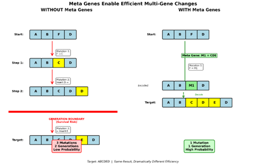
This seems like a magic bullet to the problem of search so let’s look at what’s going on. In a real-world implementation, the metagenome serves as a Lossless compression mechanism, which means the representation (a single unit) directly maps back to the multiple items it represents without any loss of information. This paired with the reduced edit distance means that a single mutation can allow for large jumps in the search space in fewer mutations.
As the metagenome grows in size and hierarchical depth it will come to capture an increasingly large volume of the search space that follows some trajectory along increasing fitness. The reduction of edit distance and the increasing number of metagenes will make the point and insert mutations disproportionately favor certain sets over others. This process continues to compound until the system reaches a singularity in probability space: a state in which all variation collapses and only a single decoded base-gene configuration retains non-zero probability of occurrence.
So, how do we fix this?
The actual answer is twofold, but I will start with my original solution and why it is not sufficient to fully explain or justify the final system.
This is where the Open mutation enters the picture.
The simplest mental model for Open comes from physics. A star becomes a black hole when it can no longer generate enough outward energy through fusion to counteract its own gravitational collapse. Once that balance is lost, compression becomes runaway.
MEGA exhibits an analogous failure mode. Metagenes introduce a powerful compressive force on representation. Information is folded inward, edit distance shrinks, and variation collapses toward reuse of increasingly abstract structures. Left unchecked, this inward pressure inevitably produces a representational singularity.
Open exists to counteract that pressure.
If metagene formation acts like gravity by pulling structure inward and increasing representational mass, then Open acts as an energetic outward force. It locally reverses compression, re-exposing internal structure and restoring degrees of freedom that would otherwise be lost.
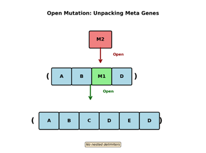
Open is exactly the inverse operation of capture. Take the M2 metagene that we have been working with for a while now. If an open mutation triggers on top of it, the capture sequence is reversed only on that individual occurrence of M2. The sequence is unpacked, and delimiters are placed around it, creating the sequence (A B M1 D). which if you remember decodes back to ABCDED. Now since this has a nested metagene within it, if another open mutation were to occur on M1, it would be unpacked back to CDE. However, in this case delimiters are not included to preserve our no nesting of delimiters rule. That’s it there is nothing else that Open does except undo the capture mutation.
Note: This does not impact other instances of the metagene being mutated. It also does not modify the metagenome in any way. What this accomplished is that it allows the algorithm to have the capacity to move up and down the hierarchy allowing us to act on the representation at various levels of granularity. The no duplicate capture rule prevents the freshly opened metagene from being recaptured without being modified in some way that changes the information or structure it contains.
Above, I pointed out that the solution to the singularity problem is twofold and it is for a very specific reason this is because open doesn’t directly modify the metagenome or the population. Doing so would be extremely difficult to implement on a computer without excessive computation. Doing so would also violate something more fundamental; the principle of locality. This is a fancy way of saying that the effect directly follows from the cause. If we allow for open to impact the metagenome or the population, we’re essentially saying a local cause directly has a non-local impact which doesn’t make any sense.
The LRU Cache
To fully address this, we also need to introduce another element of the system: the Least Recently Used (LRU) Cache.
Note: over the development of MEGA the LRU was originally used like all caches, to improve efficiency by holding on to frequently used information. The need for a cache in MEGA is slightly different. Typically, Caches are used to hold commonly accessed data for quick loading. In MEGA the data structures are not heavy in storage or load time.
Rather, when a metagene is decoded, it is potentially a deep multi-layered process that takes time. Instead of storing just the data we need to access we store the encoding alongside the decided value. This way we can just look up the Encoding token and immediately see what its decoded value is without the cost of decoding its value through the hierarchy.
I originally only used it this way until the singularity problem combined with the infinite growth of the metagenome revealed itself as a persistent failure mode. Then the LRU was adapted to include memory management. At this point it became something more than just a Cache. It became a part of the system dynamics that drive it functioning. I will properly explain this as we go but I first need to explain how it originally worked before I implemented deletion, so it is clear why deletion became a necessary addition.
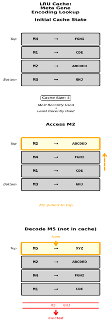
So, the LRU Cache can be thought of as a stack of Encodings and the values that they map back to. Each time an encoding is used, if it is in the Cache, it gets pulled from its position in the stack and moved to the top of the stack. So, at any given time the stack reflects an ordering of metagenes from the most recently used down to the least recently used. If there are more metagenes than the LRU has size to accommodate when a metagene outside of the LRU is decoded, we need to go through the algorithmic decoding process described above to get its decoded value which is expensive. That encoding and its decode value are then put on the top of the Cache and the bottom element falls out.
Since there are potentially infinite metagenes we face a choice with only one real answer. Either we predefine the LRU size before we run the algorithm and hope that we don’t overshoot it before the end of the run. Or we have the cache grow along with the size of the metagenome which creates a problem we can’t exactly fix. In a long run where the metagenome could potentially grow to thousands of metagenes each new metagene means the LRU cache is longer and lookup times increase, so does the amount of storage required to hold it. This essentially defeats the point of a caching system by definition and would absolutely fail if MEGA were ever deployed as an always on system.
This leaves us facing a limited Cache size and another problem that I knew was going to happen but put off fixing for way too long. Say we have a preset cache of 100 slots, and we end up with something like 200 metagenes. Each metagene that is not held in the cache needs to be decoded rather than simply looked up. If we have a purely uniform random choice in picking metagenes from the metagenome for use in mutations our odds are 50/50 that the chosen metagene is in the cache. If we consider that the population only favors metagenes that are currently contributing to fitness the odds are a bit higher that a gene being decoded is already in the cache. As the number of metagenes increases though it becomes increasingly likely that metagenes selected for use are not in the LRU cache and possibly not in use in the population at all. Which means we’re now favoring metagenes that aren’t naturally occurring within the population in favor of metagenes that have been discarded by evolution in favor of newer versions. This also has the consequence of doing more work decoding metagene mappings instead of looking them up in the cache and that’s a problem. It makes everything run slower and wastes time testing and rejecting metagenes that are likely no longer relevant to the current population’s current state.
The fix for this isn’t exactly obvious but if you think about it, it makes a lot of sense. This is not entirely dissimilar to the problem of choosing between Base gene and metagene. The key difference is when selecting a Gene for a point of insert mutation we’re choosing this kind of gene or that kind of gene. In the case of metagenes, it’s different because the choice isn’t between their classes; rather, it’s between their occurrence by order of time. A simple mental example of this is: say we’re driving a car down a gravel road; we might slow down. Then when it turns from gravel to pavement, we don’t change our speed or driving style at all. That might seem like something stupid to do, and you would be right.
The case is the same for MEGA. The population can be seen as a vehicle driving down the road and its current state reflects the current circumstances in its environment. The fitness function. As it moves forward in time it changes its location in the search space and old adaptations might not be relevant, but in the case of the LRU we’re constantly taking old patterns and applying them to the population as if they still matter, which makes driving more difficult and inefficient.
The solution to this speaks to but ultimately fails to address those multiple loose ends that we left hanging above.
Warning: So far, every problem has had a fairly intuitive explanation for its justification and how it addresses the problem directly. From here on things get a little messier. Because up until now everything has been very local; X causes Y which in turn has Z consequences. Everything has been local, and we hit a point where problems were starting to branch. Not because something is fundamentally broken but because MEGA is a closed system where there are multiple smaller interacting systems that feed into and collectively construct an object (the metagenome) which in turn touches everything else. From here on out we are looking at the global picture that ties everything else together so those small local consequences can propagate and have global consequences for the system and themselves. Translation: Things get a little messier from here out.
Part of the solution to the above is, we stop using metagenes uniformly. Instead, we keep track of their order of appearance. When we make the decision to use a metagene for a point of insert mutation, we preferentially select newer metagenes over older. As more metagenes appear older ones exponentially lose their preference. This means metagenes that recently appeared are used in the current context from which they recently appeared. This also has the consequence of newer metagenes being more likely to be nested within slightly older metagenes which are themselves further nested within slightly older metagenes. It also makes it more likely that slightly older metagenes will be contained in slightly newer metagenes. It also means that aging metagenes have an opportunity to prove themselves relevant in the current context of the state space through becoming nested in newer/ slightly older metagenes. It has the consequence of pushing the Hierarchy towards greater depth. When you take into consideration the value of the probability of choosing a metagene vs a Base gene you can easily see that we can control the pressure we place on the hierarchy. Through favoring metagenes more than Base genes we create the conditions for increasing or decreasing nesting.
We have reached the point where I stopped tinkering with MEGA and started testing what it was capable of. Conceptually everything is there or at least I thought.
I was aware of the Infinity problem and the singularity problem but didn’t realize how much of an impact it would have on the overall functioning of the system. Sometimes it would work great other times it would work terrible. Then I would tune it, and the problem would change and ultimately, I started running into crashes on longer runs which were obviously because the metagenome was getting too large to handle. I had been putting off working out deletion for a long time but if I wanted to take this to completion, I needed to get this figured out.
You might think the car analogy above was a little loose, and you would be right. I mean who would be dumb enough to let a GA drive a car right? But it begs a subtle but important question. Given the global task of driving down a road, how do you adjust your behavior to the current road conditions without risking the global goal of successfully driving the car to its destination? Driving a car is driving a car no matter what conditions you face on the road. However, going from gravel to snow to ice changes the subtleties of how you accelerate, steer, and counter-steer to not crash. Right now, this is an equivalent problem to what we face in our algorithm in its current form.
The exponential decay of metagene selection addresses the problem of maintaining the use and creation of new metagenes that change frequency as the population traverses the search space. But how can we safely delete a metagene without messing everything else up?
Before we dig deeper into that we need to be explicitly aware of the properties of the metagenome that will be affected if say a random metagene was just removed.
Metagenes are compositional structures that are represented by a unique identifier which contains their mappings.
Example:
M1 > CDE, M2 > ABM1D. If we were to delete M1, then when we decode M2 we don’t have access to the content of M1 anymore so decoded value of M2 which existed at its creation would be disrupted by the absence of M1.
The metagenome may be a global product of all sub parts and their actions but that does not mean it has global reach that can violate locality and or causality. Translation: The metagenome is global in the sense that other systems construct it from their functioning while its existence actively influences the functioning of the systems which create it. Despite that, the metagenome itself is a distinct object with its own local properties. Changing something within the metagenome should only immediately impact the properties of itself. All other effects should be realized downstream through the various interfaces the metagenome has with other systems.
In short, the current state of the solution is already decided. What’s done is done. Changing its state in a way that doesn’t directly follow from a cause that it is in contact with violates locality and is not allowed.
I realize that this might feel like an arbitrary choice given this is a computation which does in fact have the capacity to reach out and globally modify information. However, if you consider that locality is enforced because any non-local correction requires an external model of value, which MEGA is explicitly designed not to assume. Then it starts to make sense.
Ok so now that we understand what constraints we need to respect; how can we identify which metagenes should be deleted, and which ones should be left alone?
We have the LRU cache which is a container that does two things. One increases decoding speed through maintaining a mapping of encodings to decoded values and two orders them according to most recent usage. We know that the LRU has a capacity, and that the metagenome grows without an enforced upper bound. Eventually there will come a point where the metagenome is too large for the LRU to hold. This justifies the creation of a new container which the overflow can fall into when it gets pushed out of the LRU. This is where metagenes get to meet the reaper in the form of the deletion basket.
The deletion basket is a space where no metagene is safe to just hang out for free. If a metagene stays in the deletion basket for more than two generations, it will be deleted.
Why two generations?
Well, if you remember when a metagene is decoded it updates in the LRU by being moved to the top of the stack. The only time any given metagene has the possibility of being decoded is at the evaluation stage of the GA loop when we evaluate the population against the fitness function to assign the fitness value. Any metagene being actively used within the population will have its position in the LRU updated. If the metagenome is larger than the LRU what is left in the deletion basket is what simply doesn’t fit inside of the LRU and says nothing about existence in the population. However, the next time the population is decoded in the next generation metagenes that cycle into and back out of the LRU have their counter reset but the ones that are genuinely unused within the population are at the value of 2. This proves that they were not decoded this evaluation making them safe to delete without having global consequences to the population’s decoded identity. So now that we understand how to identify metagenes that will be deleted, how do we go about the actual process?
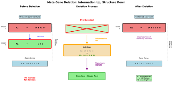
The answer to this comes from the properties of the DAG data structure. Since the Structure of a DAG goes in one direction with no loops, each metagene can be decoded by following the mappings from one metagene down to the next until it comes to the base level. That means any nested metagene has a link from itself up to the genes that contain it. When we delete a metagene, we first ask what is its content? We take its content and check all other metagenes and see which ones map back to the metagene being deleted. We then replace their references with the content of the metagene being deleted. This process is known as inlining.
Example:
Let’s return to the example we have been working with from the start.
Reminder:
- Our base genes are ABCDEFGHIJ
- M1 maps to CDE
- M2 maps to (A B M1 D) which decodes to ABCDED
Let’s say M1 gets identified for deletion. We then identify the content of M1 which is CDE. You then look at the Genes in the metagenome looking for the ones that contain M1 which would be M2. We then modify M2 replacing the reference to M1 with CDE and M2 now decodes to ABCDED.
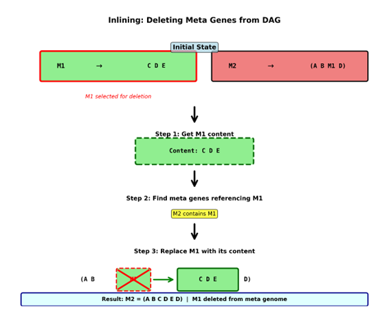
Once deletion is complete the Encoding for M1 gets put into the reuse pool freeing up the encoding to be reused without creating any conflicts because all its prior references have been replaced with its unpacked content through inlining.
The above is just a baby example of this process in action to demonstrate what happens and something that is important to take note of is the effect that this has on gene ordering if you remember M1 was order 1 and M2 was order 2. Now that M1 has been deleted M2 is now order 1. This is important to understand because on a larger scale you can see how this has consequences that feed back into the population. Deletion flattens hierarchy and at the same time pushes information upwards in the hierarchy.
Now this ultimately brings us back to the open mutation which we previously left hanging as an incomplete answer to the problem of singularity formation. So, let’s put them together. Metagene deletion globally flattens the hierarchy but is limited to acting only on the metagenome. Metagenes enter the population through mutation as compressed units. Over time those units change their internal structure which is invisible to the Population through inlining preserving their identity. Deletion pushes information upward and flattens structure. This is where exponential decay of metagene selection preference becomes important. It essentially says that so long as we are continually generating new metagenes that already existing metagenes become less valuable. They eventually stop being inserted into the population and must survive by being useful to the organisms they already exist in as they reproduce. If they fail to do so they will fall out of the population and be deleted. However, their information survives through inlining into newer metagenes, but which now have a flatter structure. So only valuable metagenes can become deeply embedded in the hierarchy where less valuable metagenes have a shallow nesting making them less protected in the presence of the open mutation. Given that a metagene can’t be opened and immediately recaptured as a duplicate they are forced to be modified. This means that a less valuable metagenes information is both at an increasingly likely risk of being deleted but it also has an increasingly high risk of being cracked open which re-exposes the information to mutation and enforced modification. Which means that information must continually justify its own existence or face deletion or refinement under the current population’s location in the state space.
This creates something called self-evidencing. Where an abstraction must continuously prove and justify its own continued existence to the system. Yes, the definition implies agency among other things. As invoked here I simply mean to justify your continued existence you must provide evidence of your value to the system. In this specific case the Evidence is the metagenes proof of usage within the population. In the face of exponential decay in usage through point and insert mutations any single metagene will eventually have to persist through being contained within organisms who survive the GA loop. Otherwise, it will be deleted and the information it contains diffused up into the hierarchy, to be further refined and evaluated by the battlefield of Evolution.
Ok we have covered the SGA mutations and a few of the MEGA-specific mutations. There is one more left uncovered
Don’t worry, this isn’t a lead into another 10 pages of explanation. All of this had to be explained before it made sense to conclude with the final mutation.
So far, we have:
- Insert delimiter pair -> Creates new delimiters.
- Capture -> removes delimiters.
- Open -> creates new delimiters.
We’re missing one. Open is offset by Capture (which removes delimiters) but Insert Delimiter Pair increases delimiter pairs with no counter force. Eventually Delimiters will saturate. Dividing the population into segments that aren’t easy to mix or act on through mutation or crossover. So, we introduce Delimit Delete, which does exactly that: it deletes delimiters from the population and has its own parameter-controlled probability. This offsets the effects of insert delimiter pair keeping the whole system in balance preventing runaway degradation.
From here we have tied every local consequence that leads to pathological failure into a global product of the system whose mechanisms address those failure modes and feed the outcome back into the dynamics of the system effectively closing the loop.
I realize this has been a very long and involved walkthrough of the whole of MEGA. This format was chosen because despite making use of the Standard GA loop MEGA is not a GA. MEGA is a closed dynamical system that also happens to be useful for performing work. It is primarily composed of two layers (the GA loop and the metagenome) enabled by the MEGA-specific mutations. These additions to the SGA together with their constraints create a complex interplay between the SGA loop and the metagenome. This interplay is composed of multiple coupled sub systems and feedback loops which enable it to function without exploding.
Ideally MEGA should be taken as a whole. So, to finish this out I’d like to briefly go over a few key points.
I realize that the strict enforcement of locality may feel like a choice, but in the context MEGA, it is a functional requirement. Locality is the barrier that prevents MEGA from collapsing into a traditional, hand-tuned heuristic.
If we allowed for non-local corrections, such as reaching into the population to ‘fix’ representations after a metagene is deleted, we would be forced to introduce an external model of value. This would require the engine to make assumptions about the state of the search that it simply can’t make without resorting to a more complicated and fragile method of explicit control. By enforcing locality, we ensure that simplicity is maintained and that the system remains open-ended. The dynamics are allowed to resolve themselves through interaction rather than being steered by top-down intervention. In MEGA, locality is not just a principle; it is the mechanism that ensures the hierarchy is a genuine emergent product of the system’s own internal logic.
Next Exponential Decay of the metagenes should not be viewed as a ticking clock. It is an event-driven mechanism driven by the current number of metagenes in the Population. Each new metagene makes the ones below increasingly less likely to be selected for use in a point or insert mutation. It is not driven by cycles. It is driven by the creation of new metagenes which may or may not happen at regular intervals.
I realize that invoking self-evidencing is an incredibly strong claim and demands explanation and evidence. The next release behind this one will be a theoretical document paired with the PFOL specification that should make the justification of this seem clearer and more reasonable. After that will follow falsifiable Experimental results. In this document itself I feel I have done a reasonable job of hinting at the justification in a way that would not be overwhelming to a non-technical reader and that is intentional. At this point my aim is to build an intuition about MEGA to avoid category error by assumption with SGAs.
In conclusion to answer the titled question. What kind of thing is MEGA?
MEGA is not simply a genetic algorithm, nor is it a static optimization method. It is a system in which representations, abstractions, and memory structures evolve under locality and bounded constraints. The mechanisms described above collectively define a class of systems in which internal structure is generated and maintained through adaptive dynamics rather than explicit control.
In subsequent theoretical work, I will refer to this class as Generative Adaptive Dynamical Systems (GADS). MEGA is presented here as the first concrete instantiation of this class.
If you have made it this far without throwing your hands up and walking away… Thank-you for your time and patience. I hope this helped to give you a clearer intuition about the inner workings of MEGA. I am very passionate about my work and am excited to keep pushing forward into the unknown.
Thank you for your support.